Clasificación de moda con Pytorch

Escrito por
20 minutos de lectura
Cargar los datos
# our basic libraries
import torch
import torchvision

# data loading and transforming
from torchvision.datasets import FashionMNIST
from torch.utils.data import DataLoader
from torchvision import transforms

# The output of torchvision datasets are PILImage images of range [0, 1].
# We transform them to Tensors for input into a CNN

## Define a transform to read the data in as a tensor
data_transform = transforms.ToTensor()

# choose the training and test datasets
train_data = FashionMNIST(root='./data', train=True,
                                   download=True, transform=data_transform)

test_data = FashionMNIST(root='./data', train=False,
                                  download=True, transform=data_transform)


# Print out some stats about the training and test data
print('Train data, number of images: ', len(train_data))
print('Test data, number of images: ', len(test_data))
Train data, number of images:  60000
Test data, number of images:  10000
batch_size = 20

train_loader = DataLoader(train_data, batch_size=batch_size, shuffle=True)
test_loader = DataLoader(test_data, batch_size=batch_size, shuffle=True)

# specify the image classes
classes = ['T-shirt/top', 'Trouser', 'Pullover', 'Dress', 'Coat',
           'Sandal', 'Shirt', 'Sneaker', 'Bag', 'Ankle boot']
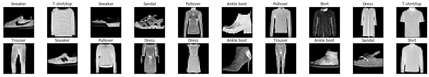
Visualizar algunos datos de entrenamiento
import numpy as np
import matplotlib.pyplot as plt

%matplotlib inline

# obtain one batch of training images
dataiter = iter(train_loader)
images, labels = dataiter.next()
images = images.numpy()

# plot the images in the batch, along with the corresponding labels
fig = plt.figure(figsize=(25, 4))
for idx in np.arange(batch_size):
    ax = fig.add_subplot(2, batch_size/2, idx+1, xticks=[], yticks=[])
    ax.imshow(np.squeeze(images[idx]), cmap='gray')
    ax.set_title(classes[labels[idx]])
Definir la arquitectura de la red
import torch.nn as nn
import torch.nn.functional as F

class Net(nn.Module):

    def __init__(self):
        super(Net, self).__init__()

        # 1 input image channel (grayscale), 10 output channels/feature maps
        # 3x3 square convolution kernel
        self.conv1 = nn.Conv2d(1, 10, 3)

        # Maxpooling layer
        self.pool = nn.MaxPool2d(2, 2)

        self.conv2 = nn.Conv2d(10, 20, 3)

        # Fully-connected layer
        self.fc1 = nn.Linear(20*5*5, 50)

        # Dropout layer with a probability of an element to be zeroed of 0.4
        self.drop = nn.Dropout(p=0.4)

        # 10 Output channels (for the 10 classes)
        self.fc2 = nn.Linear(50, 10)

    def forward(self, x):
        # Two convolutional/reLu + pool layers
        x = self.pool(F.relu(self.conv1(x)))
        x = self.pool(F.relu(self.conv2(x)))

        # X Flatten
        x = x.view(x.size(0), -1)

        # Linear + Fully connected layer
        x = F.relu(self.fc1(x))

        # Dropout + Fully connected layer
        x = self.fc2(self.drop(x))

        # Softmax
        x = F.log_softmax(x, dim=1)

        # final output
        return x

# instantiate and print your Net
net = Net()
print(net)
Net(
  (conv1): Conv2d(1, 10, kernel_size=(3, 3), stride=(1, 1))
  (pool): MaxPool2d(kernel_size=2, stride=2, padding=0, dilation=1, ceil_mode=False)
  (conv2): Conv2d(10, 20, kernel_size=(3, 3), stride=(1, 1))
  (fc1): Linear(in_features=500, out_features=50, bias=True)
  (drop): Dropout(p=0.4, inplace=False)
  (fc2): Linear(in_features=50, out_features=10, bias=True)
)
Specificar la función de error (loss) y el optimizador
import torch.optim as optim

# Loss function
# The cross entropy combines softmax and NLL loss,
# so he wouldn't have to declare the softmax layer
# if we've used it
criterion = nn.NLLLoss()

# Stochastic gradient descent optimizer
optimizer = optim.SGD(net.parameters(), lr=0.001, momentum=0.9)
Precisión
# Calculate accuracy before training
correct = 0
total = 0

# Iterate through test dataset
for images, labels in test_loader:

    # forward pass to get outputs
    # the outputs are a series of class scores
    outputs = net(images)

    # get the predicted class from the maximum value in the output-list of class scores
    _, predicted = torch.max(outputs.data, 1)

    # count up total number of correct labels
    # for which the predicted and true labels are equal
    total += labels.size(0)
    correct += (predicted == labels).sum()

# calculate the accuracy
accuracy = 100 * correct.item() / total

# print it out!
print('Accuracy before training: ', accuracy)
Accuracy before training: 9.02
Entrenar la red
def train(n_epochs):

    loss_over_time = [] # to track the loss as the network trains

    for epoch in range(n_epochs):  # loop over the dataset multiple times

        running_loss = 0.0

        for batch_i, data in enumerate(train_loader):
            # get the input images and their corresponding labels
            inputs, labels = data

            # zero the parameter (weight) gradients
            optimizer.zero_grad()

            # forward pass to get outputs
            outputs = net(inputs)

            # calculate the loss
            loss = criterion(outputs, labels)

            # backward pass to calculate the parameter gradients
            loss.backward()

            # update the parameters
            optimizer.step()

            # print loss statistics
            # to convert loss into a scalar and add it to running_loss, we use .item()
            running_loss += loss.item()

            if batch_i % 1000 == 999:    # print every 1000 batches
                avg_loss = running_loss/1000
                # record and print the avg loss over the 1000 batches
                loss_over_time.append(avg_loss)
                print('Epoch: {}, Batch: {}, Avg. Loss: {}'.format(epoch + 1, batch_i+1, avg_loss))
                running_loss = 0.0

    print('Finished Training')
    return loss_over_time
n_epochs = 30

training_loss = train(n_epochs)
Epoch: 1, Batch: 1000, Avg. Loss: 1.7501887657642365
Epoch: 1, Batch: 2000, Avg. Loss: 0.9992681905925274
Epoch: 1, Batch: 3000, Avg. Loss: 0.9019102705419063
Epoch: 2, Batch: 1000, Avg. Loss: 0.8175063020586968
Epoch: 2, Batch: 2000, Avg. Loss: 0.7706369262635708
Epoch: 2, Batch: 3000, Avg. Loss: 0.7071908851563931
Epoch: 3, Batch: 1000, Avg. Loss: 0.6741744703352451
Epoch: 3, Batch: 2000, Avg. Loss: 0.6341438280940056
Epoch: 3, Batch: 3000, Avg. Loss: 0.6152339836359024
Epoch: 4, Batch: 1000, Avg. Loss: 0.604816315099597
Epoch: 4, Batch: 2000, Avg. Loss: 0.572301662042737
Epoch: 4, Batch: 3000, Avg. Loss: 0.5713251649439335
Epoch: 5, Batch: 1000, Avg. Loss: 0.5569603327736259
Epoch: 5, Batch: 2000, Avg. Loss: 0.5404066774919629
Epoch: 5, Batch: 3000, Avg. Loss: 0.5368393697589636
Epoch: 6, Batch: 1000, Avg. Loss: 0.5234340626597405
Epoch: 6, Batch: 2000, Avg. Loss: 0.5098866861164569
Epoch: 6, Batch: 3000, Avg. Loss: 0.5071937583684921
Epoch: 7, Batch: 1000, Avg. Loss: 0.4946084372624755
Epoch: 7, Batch: 2000, Avg. Loss: 0.49338393967598676
Epoch: 7, Batch: 3000, Avg. Loss: 0.4859438165351748
Epoch: 8, Batch: 1000, Avg. Loss: 0.47368826558440924
Epoch: 8, Batch: 2000, Avg. Loss: 0.4712853904888034
Epoch: 8, Batch: 3000, Avg. Loss: 0.4668237509354949
Epoch: 9, Batch: 1000, Avg. Loss: 0.4670602819994092
Epoch: 9, Batch: 2000, Avg. Loss: 0.45304538125172256
Epoch: 9, Batch: 3000, Avg. Loss: 0.44266059119254353
Epoch: 10, Batch: 1000, Avg. Loss: 0.43968673377484085
Epoch: 10, Batch: 2000, Avg. Loss: 0.4464306502379477
Epoch: 10, Batch: 3000, Avg. Loss: 0.4383479151129723
Epoch: 11, Batch: 1000, Avg. Loss: 0.42926819264143706
Epoch: 11, Batch: 2000, Avg. Loss: 0.4281160565726459
Epoch: 11, Batch: 3000, Avg. Loss: 0.4367229501605034
Epoch: 12, Batch: 1000, Avg. Loss: 0.41990946324914696
Epoch: 12, Batch: 2000, Avg. Loss: 0.41516623869538305
Epoch: 12, Batch: 3000, Avg. Loss: 0.4294245415255427
Epoch: 13, Batch: 1000, Avg. Loss: 0.41292278353124856
Epoch: 13, Batch: 2000, Avg. Loss: 0.42076494720205665
Epoch: 13, Batch: 3000, Avg. Loss: 0.4065509000942111
Epoch: 14, Batch: 1000, Avg. Loss: 0.40586154959350823
Epoch: 14, Batch: 2000, Avg. Loss: 0.4023443521186709
Epoch: 14, Batch: 3000, Avg. Loss: 0.40409189872816204
Epoch: 15, Batch: 1000, Avg. Loss: 0.3990190891176462
Epoch: 15, Batch: 2000, Avg. Loss: 0.3889594701286405
Epoch: 15, Batch: 3000, Avg. Loss: 0.395684513553977
Epoch: 16, Batch: 1000, Avg. Loss: 0.3949708788692951
Epoch: 16, Batch: 2000, Avg. Loss: 0.3816620577275753
Epoch: 16, Batch: 3000, Avg. Loss: 0.38925764700397847
Epoch: 17, Batch: 1000, Avg. Loss: 0.3762176215797663
Epoch: 17, Batch: 2000, Avg. Loss: 0.3873607496935874
Epoch: 17, Batch: 3000, Avg. Loss: 0.3856014817915857
Epoch: 18, Batch: 1000, Avg. Loss: 0.38045168679580094
Epoch: 18, Batch: 2000, Avg. Loss: 0.37652721055410804
Epoch: 18, Batch: 3000, Avg. Loss: 0.37830156134068965
Epoch: 19, Batch: 1000, Avg. Loss: 0.3707478314563632
Epoch: 19, Batch: 2000, Avg. Loss: 0.3751325882524252
Epoch: 19, Batch: 3000, Avg. Loss: 0.3620608055330813
Epoch: 20, Batch: 1000, Avg. Loss: 0.3679933508746326
Epoch: 20, Batch: 2000, Avg. Loss: 0.36531098840385673
Epoch: 20, Batch: 3000, Avg. Loss: 0.3664118441361934
Epoch: 21, Batch: 1000, Avg. Loss: 0.36158943648543207
Epoch: 21, Batch: 2000, Avg. Loss: 0.3611026970297098
Epoch: 21, Batch: 3000, Avg. Loss: 0.36100602328404785
Epoch: 22, Batch: 1000, Avg. Loss: 0.3503793747276068
Epoch: 22, Batch: 2000, Avg. Loss: 0.36088213962875304
Epoch: 22, Batch: 3000, Avg. Loss: 0.3527381945550442
Epoch: 23, Batch: 1000, Avg. Loss: 0.35468466183170677
Epoch: 23, Batch: 2000, Avg. Loss: 0.35481646746769546
Epoch: 23, Batch: 3000, Avg. Loss: 0.35257206600904467
Epoch: 24, Batch: 1000, Avg. Loss: 0.3397639312148094
Epoch: 24, Batch: 2000, Avg. Loss: 0.35246075225248935
Epoch: 24, Batch: 3000, Avg. Loss: 0.3447857304476202
Epoch: 25, Batch: 1000, Avg. Loss: 0.3410695663690567
Epoch: 25, Batch: 2000, Avg. Loss: 0.3413340912982821
Epoch: 25, Batch: 3000, Avg. Loss: 0.3411646853480488
Epoch: 26, Batch: 1000, Avg. Loss: 0.3371873890273273
Epoch: 26, Batch: 2000, Avg. Loss: 0.3324272054824978
Epoch: 26, Batch: 3000, Avg. Loss: 0.3410472013764083
Epoch: 27, Batch: 1000, Avg. Loss: 0.33442076738364995
Epoch: 27, Batch: 2000, Avg. Loss: 0.3444551220955327
Epoch: 27, Batch: 3000, Avg. Loss: 0.3285349723454565
Epoch: 28, Batch: 1000, Avg. Loss: 0.3229098819456995
Epoch: 28, Batch: 2000, Avg. Loss: 0.34214119989424946
Epoch: 28, Batch: 3000, Avg. Loss: 0.33388355425558985
Epoch: 29, Batch: 1000, Avg. Loss: 0.3306284485906362
Epoch: 29, Batch: 2000, Avg. Loss: 0.33167849070206284
Epoch: 29, Batch: 3000, Avg. Loss: 0.32657250584475694
Epoch: 30, Batch: 1000, Avg. Loss: 0.318486179549247
Epoch: 30, Batch: 2000, Avg. Loss: 0.3298761437041685
Epoch: 30, Batch: 3000, Avg. Loss: 0.3270070698596537
Finished Training
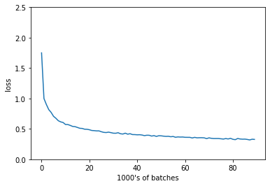
Visualizar el error
plt.plot(training_loss)
plt.xlabel("1000's of batches")
plt.ylabel("loss")
plt.ylim(0, 2.5)
plt.show()
# initialize tensor and lists to monitor test loss and accuracy
test_loss = torch.zeros(1)
class_correct = list(0. for i in range(10))
class_total = list(0. for i in range(10))

# set the module to evaluation mode
net.eval()

for batch_i, data in enumerate(test_loader):

    # get the input images and their corresponding labels
    inputs, labels = data

    # forward pass to get outputs
    outputs = net(inputs)

    # calculate the loss
    loss = criterion(outputs, labels)

    # update average test loss
    test_loss = test_loss + ((torch.ones(1) / (batch_i + 1)) * (loss.data - test_loss))

    # get the predicted class from the maximum value in the output-list of class scores
    _, predicted = torch.max(outputs.data, 1)

    # compare predictions to true label
    correct = np.squeeze(predicted.eq(labels.data.view_as(predicted)))

    # calculate test accuracy for *each* object class
    # we get the scalar value of correct items for a class, by calling `correct[i].item()`
    for i in range(batch_size):
        label = labels.data[i]
        class_correct[label] += correct[i].item()
        class_total[label] += 1

print('Test Loss: {:.6f}\n'.format(test_loss.numpy()[0]))

for i in range(10):
    if class_total[i] > 0:
        print('Test Accuracy of %5s: %2d%% (%2d/%2d)' % (
            classes[i], 100 * class_correct[i] / class_total[i],
            np.sum(class_correct[i]), np.sum(class_total[i])))
    else:
        print('Test Accuracy of %5s: N/A (no training examples)' % (classes[i]))


print('\nTest Accuracy (Overall): %2d%% (%2d/%2d)' % (
    100. * np.sum(class_correct) / np.sum(class_total),
    np.sum(class_correct), np.sum(class_total)))
Test Loss: 0.309797

Test Accuracy of T-shirt/top: 83% (831/1000)
Test Accuracy of Trouser: 97% (972/1000)
Test Accuracy of Pullover: 80% (802/1000)
Test Accuracy of Dress: 89% (892/1000)
Test Accuracy of  Coat: 88% (881/1000)
Test Accuracy of Sandal: 97% (978/1000)
Test Accuracy of Shirt: 64% (640/1000)
Test Accuracy of Sneaker: 95% (954/1000)
Test Accuracy of   Bag: 97% (976/1000)
Test Accuracy of Ankle boot: 95% (959/1000)

Test Accuracy (Overall): 88% (8885/10000)
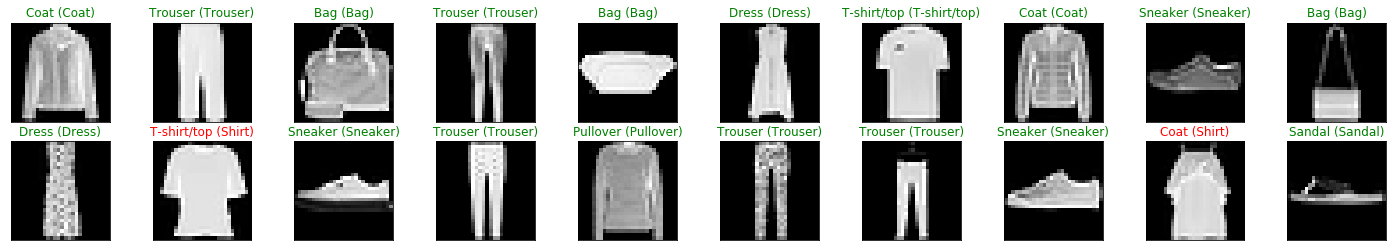
Ver algunos resultados del test
# obtain one batch of test images
dataiter = iter(test_loader)
images, labels = dataiter.next()
# get predictions
preds = np.squeeze(net(images).data.max(1, keepdim=True)[1].numpy())
images = images.numpy()

# plot the images in the batch, along with predicted and true labels
fig = plt.figure(figsize=(25, 4))
for idx in np.arange(batch_size):
    ax = fig.add_subplot(2, batch_size/2, idx+1, xticks=[], yticks=[])
    ax.imshow(np.squeeze(images[idx]), cmap='gray')
    ax.set_title("{} ({})".format(classes[preds[idx]], classes[labels[idx]]),
                 color=("green" if preds[idx]==labels[idx] else "red"))
# Saving the model
model_dir = 'saved_models/'
model_name = 'fashion_net_simple.pt'

# after training, save your model parameters in the dir 'saved_models'
# when you're ready, un-comment the line below
torch.save(net.state_dict(), model_dir+model_name)
Los resultados se podrían mejorar aumentando el número de ejemplos de T-shirt/top y coats para que así el algoritmo tuviese más datos para identificar los rasgos de ambos aunque sean muy parecidos. También podríamos añadir alguna red convolucional más para así tener mayor detalle de features que nos permitan distinguirlos.
¿Quieres contactar conmigo?
Reporta un bug
Para cualquier error en la web o en la escritura, porfavor abre un issue en Github.
GithubMándame un mensaje
Siéntete libre de mandarme un tweet con cualquier recomendación o pregunta.
Twitter